MyAutoPano
Table of Contents:
- 1. Deadline
- 2. Problem Statement
- 3. Data Collection
- 4. Phase 1: Traditional Approach
- 5. Phase 2: Deep Learning Approach
- 6. Notes about Test Set
- 7. Extra Credit
- 8. Submission Guidelines
- 9. Allowed and Disallowed functions
- 10. Collaboration Policy
- 11. Acknowledgements
1. Deadline
11:59 PM, February 24, 2024
2. Problem Statement
The purpose of this project is to stitch two or more images in order to create one seamless panorama image. Each image should have few repeated local features (\(\sim\) 30-50% or more, emperically chosen). In this project, you need to capture multiple such images. The following method of stitching images should work for most image sets but you’ll need to be creative for working on harder image sets.
3. Data Collection
As we mentioned before, you need to capture two sets of images in order to stitch a seamless panorama. Each sequence should have at-least 3 images with \(\sim\) 30-50%$$ image overlap between them. Feel free to check the sample images given to you in YourDirectoryID_p1\Phase1\Data\Train\ folder. Be sure to resize the images you capture to something manageable and place the sets respectively in YourDirectoryID_p1\Phase1\Data\Train\CustomSet1 and YourDirectoryID_p1\Phase1\Data\Train\CustomSet2. Make sure all the images are in .jpg format.
4. Phase 1: Traditional Approach
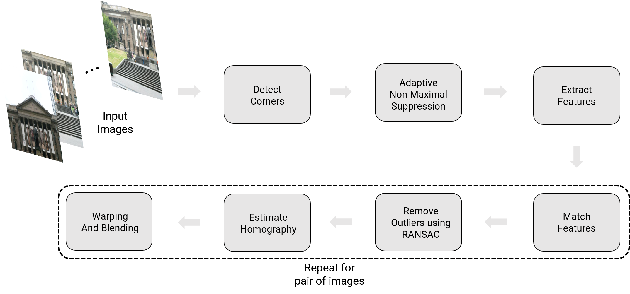
An overview of the panorama stitching using the traditional approach is given below.
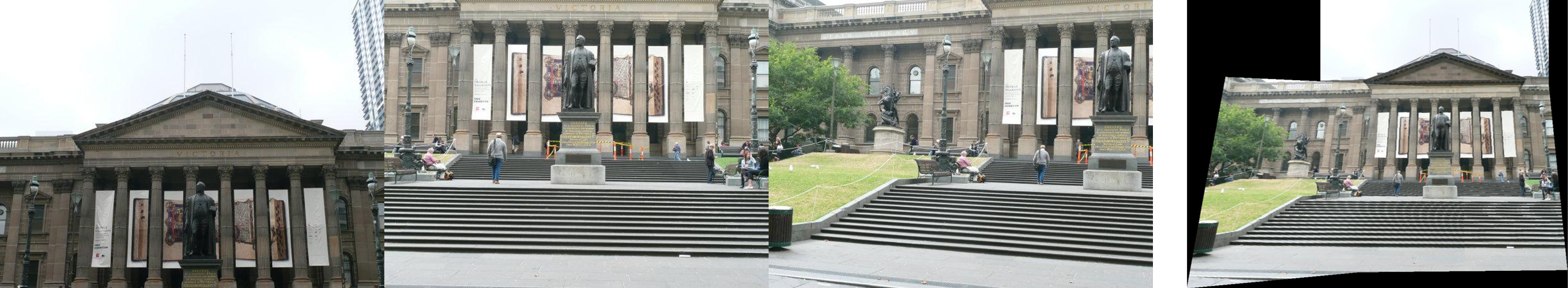
Sample input images and it’s respective output are shown below.
4.1. Corner Detection
The first step in stitching a panorama is extracting corners like most computer vision tasks. Here we will use either Harris corners or Shi-Tomasi corners. Use cv2.cornerHarris or cv2.goodFeaturesToTrack to implement this part.
4.2. Adaptive Non-Maximal Suppression (ANMS)
The objective of this step is to detect corners such that they are equally distributed across the image in order to avoid weird artifacts in warping.
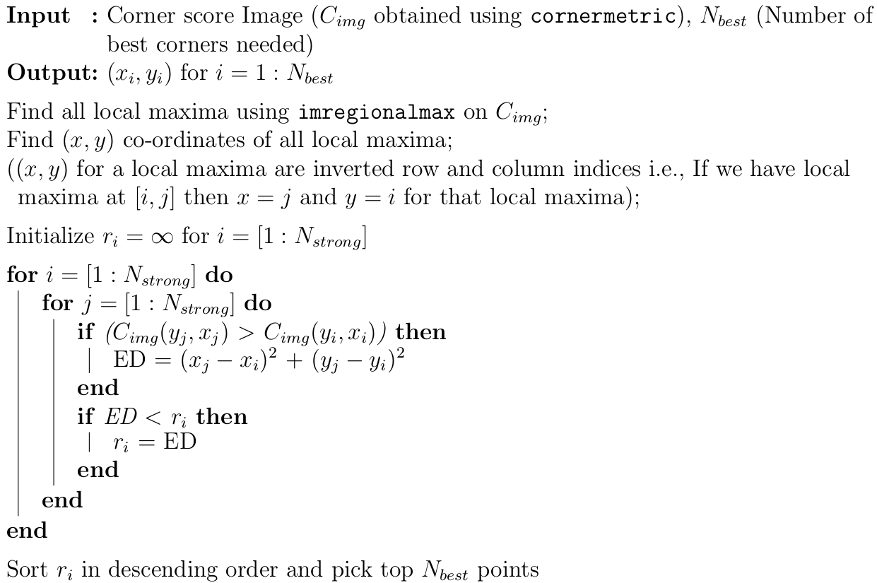
In a real image, a corner is never perfectly sharp, each corner might get a lot of hits out of the \(N\) strong corners - we want to choose only the \(N_{best}\) best corners after ANMS. In essence, you will get a lot more corners than you should! ANMS will try to find corners which are true local maxima. The algorithm for implementing ANMS is given below.
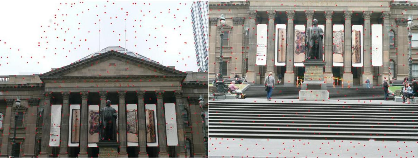
Output of corner detection and ANMS is shown below. Observe that the output of ANMS is evenly distributed strong corners.
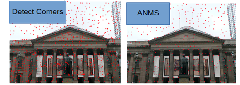
A sample output of ANMS for two different images are shown below.
4.3. Feature Descriptor
In the previous step, you found the feature points (locations of the \(N_{best}\) best corners after ANMS are called the feature point locations). You need to describe each feature point by a feature vector, this is like encoding the information at each feature point by a vector. One of the easiest feature descriptor is described next.
Take a patch of size \(40 \times 40\) centered (this is very important) around the keypoint/feature point. Now apply gaussian blur (feel free to play around with the parameters, for a start you can use OpenCV’s default parameters in cv2.GaussianBlur command. Now, sub-sample the blurred output (this reduces the dimension) to \(8 \times 8\). Then reshape to obtain a \(64 \times 1\) vector. Standardize the vector to have zero mean and variance of 1. Standardization is used to remove bias and to achieve some amount of illumination invariance.
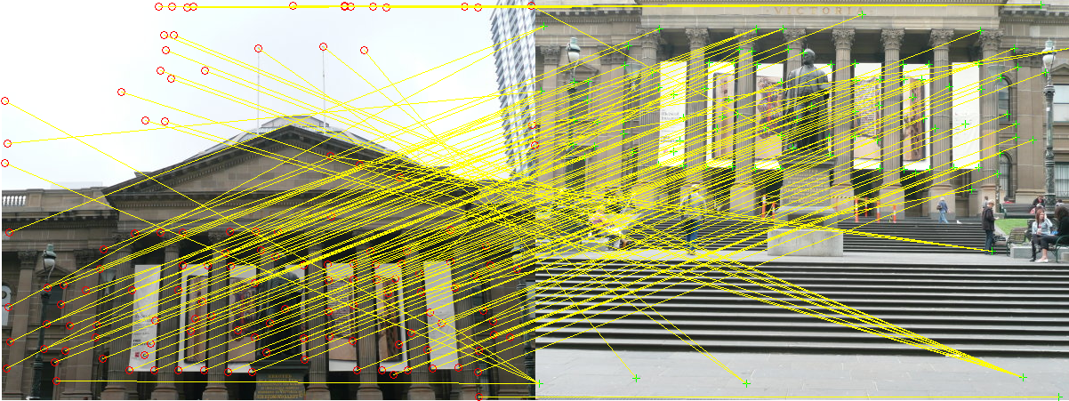
4.4. Feature Matching
In the previous step, you encoded each keypoint by \(64\times1\) feature vector. Now, you want to match the feature points among the two images you want to stitch together. In computer vision terms, this step is called as finding feature correspondences between the 2 images. Pick a point in image 1, compute sum of square differences between all points in image 2. Take the ratio of best match (lowest distance) to the second best match (second lowest distance) and if this is below some ratio keep the matched pair or reject it. Repeat this for all points in image 1. You will be left with only the confident feature correspondences and these points will be used to estimate the transformation between the 2 images, also called as Homography. Use the function cv2.drawMatches to visualize feature correspondences. Below is an image showing matched features.
4.5. RANSAC for outlier rejection and to estimate Robust Homography
We now have matched all the features correspondences but not all matches will be right. To remove incorrect matches, we will use a robust method called Random Sample Concensus or RANSAC to compute homography.
The RANSAC steps are:
- Select four feature pairs (at random), \(p_i\) from image 1, \(p_i^\prime\) from image 2.
- Compute homography \(H\) between the previously picked point pairs.
- Compute inliers where \(SSD(p_i^\prime, Hp_i) < \tau\), where \(\tau\) is some user chosen threshold and \(SSD\) is sum of square difference function.
- Repeat the last three steps until you have exhausted \(N_{max}\) number of iterations (specified by user) or you found more than some percentage of inliers (Say \(90\%\) for example).
- Keep largest set of inliers.
- Re-compute least-squares \(\hat{H}\) estimate on all of the inliers.
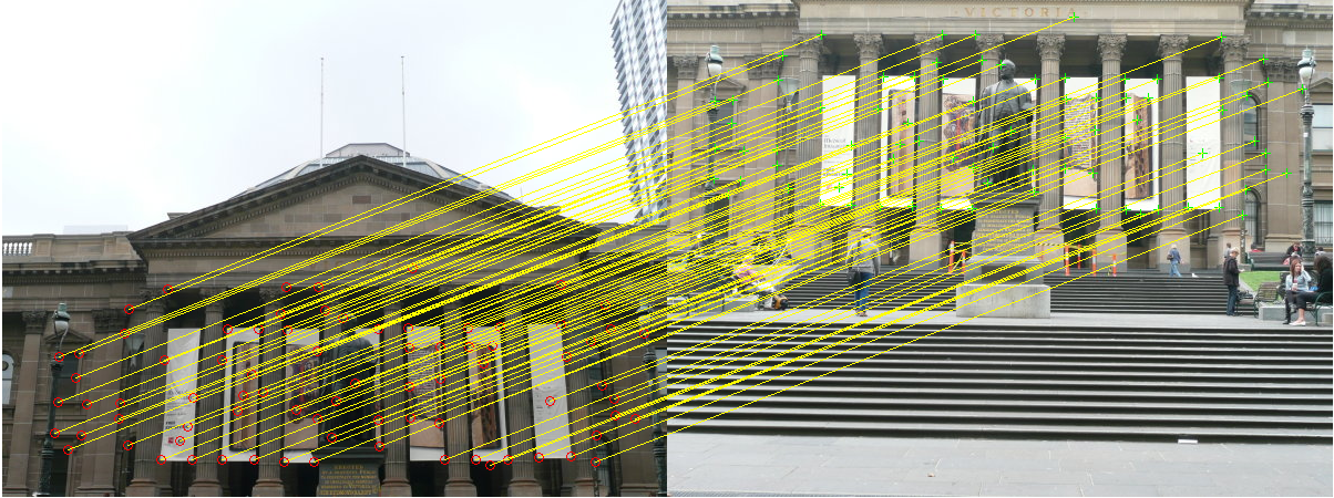
The output of feature matches after all outliers have been removed is shown below.
4.6. Blending Images
Panorama can be produced by overlaying the pairwise aligned images to create the final output image. The output panorama stitched from two images shown in the Fig. 6 are shown below.
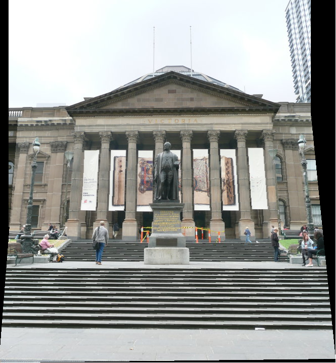
Come up with a logic to blend the common region between images while not affecting the regions which are not common. Here, common means shared region, i.e., a part of first image and part of second image should overlap in the output panorama. Describe what you did in your report. Feel free to use any built-in or third party code for blending to obtain pretty results.
Note: The pipeline talks about how to stitch a pair of images, you need to extend this to work for multiple images. You can re-run your images pairwise or do something smarter. Your end goal is to be able to stitch any number of given images - maybe 2 or 3 or 4 or 100, your algorithm should work. If a random image with no/less number matches are given in a set, your algorithm needs to not use them in the final panorama. If all the images have no common features/low number of common features then report an error.
Note: When blending these images, there are inconsistency between pixels from different input images due to different exposure/white balance settings or photometric distortions or vignetting. This can be resolved by Poisson blending. Feel free to use any built-in or third party code for Poisson blending to obtain pretty results.
An input and output of a seamless panorama of three images are shown below.
5. Phase 2: Deep Learning Approach
You are going to be implementing two deep learning approaches to estimate the homography between two images. The deep model effectively combines corner detection, ANMS, feature extraction, feature matching, RANSAC and estimate homography all into one. This not only makes the approach faster but also makes it robust if the network is generalizable (More on this later).
5.1. Data Generation
To train a Convolutional Neural Network (CNN) to estimate homography between a pair of images (we call this network HomographyNet and the original paper can be found here) we need data (pairs of images) with the known homogaraphy between them. This is in-general hard to obtain as we would need the 3D movement between the pair of images to obtain the homography between them. An easier option is to generate synthetic pairs of images to train a network. But what images do we use so that the network is not baised? Simple, use images from MSCOCO dataset which contains images of a lot of objects in natural scenes. MSCOCO is quite large and it’ll take forever to train on these images. Hence, we provide a small subset of MSCOCO for you to train your HomographyNet on. This dataset is included with your starter code in the YourDirectoryID_p1\Phase2\Data\ folder, this folder contains both Train and Val images in their respective folders.
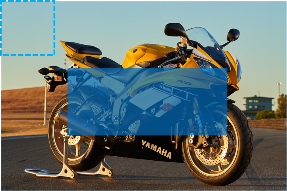
Now that you’ve downloaded the dataset, we need to generate synthetic data, i.e., pairs of images with known homography between them. Before, we generate image pairs, we need all the image pairs to be of the same size (as HomographyNet is not fully convolutional, it cannot accept image sizes of arbitrary shape). First step in generating data is to obtain a random crop of the image (called patch). Then the original image will be warped using a random homography and finally the respective patch on the warped image is extracted. While we perform this operation we need to ensure that we are not extracting the patch from outside the image after warping. An illustration is shown below.
Let’s go through the steps of generating data now.
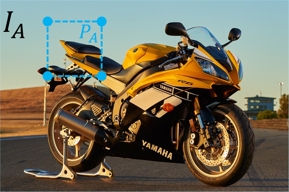
Step 1
Obtain a random patch (\(P_A\) of size \(M_P\times N_P\)) from the image (\(I_A\)) of size \(M\times N\)) with \(M>M_P\) and \(N>N_P\) such that all the pixels in the patch will lie within the image after warping the random extracted patch. Think about where you have to extract the patch \(P_A\) from \(I_A\) if maximum possible perturbation is in \([-\rho, \rho]\).
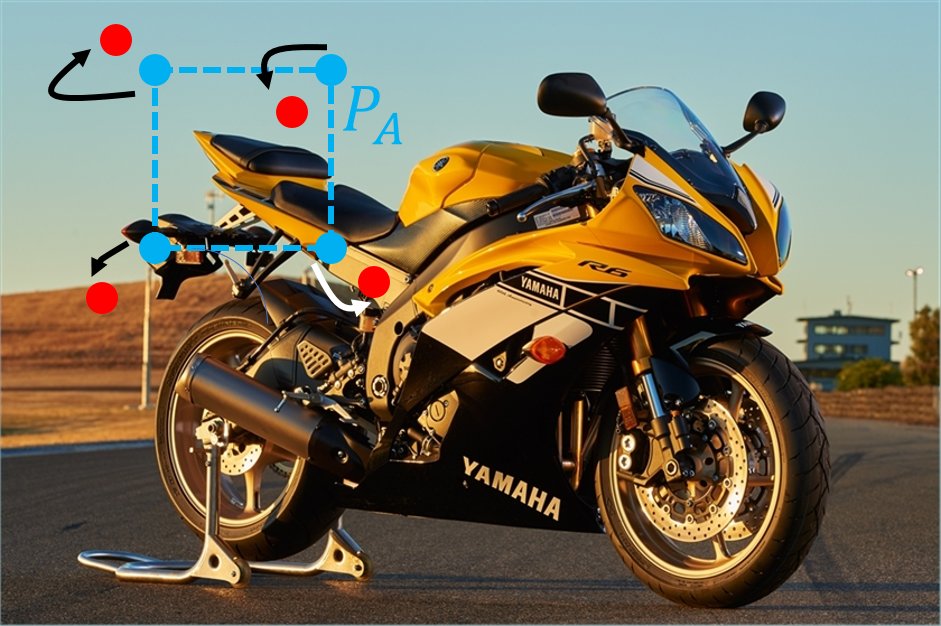
Step 2
Perform a random perturbation in the range \([-\rho, \rho]\) to the corner points (top left corner, top right corner, left bottom corner and right bottom corner – not the corners in computer vision sense) of \(P_A\) in \(I_A\). This is illustrated in the figures below.
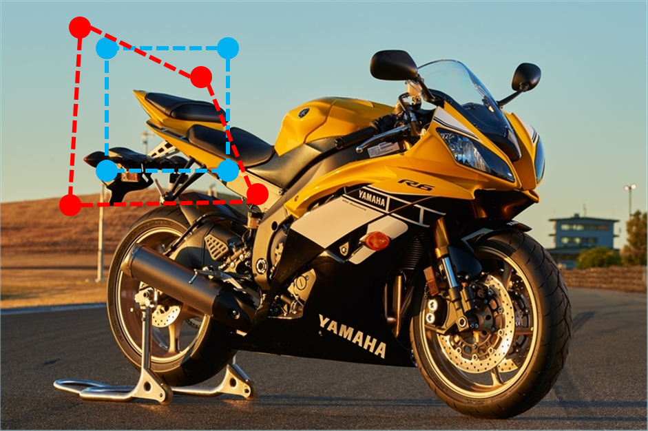
As mentioned in the last figure, we want to extract data such that we add minimal amount of extra data and we don’t want to mask anything or add black pixels (pixels outside image assuming zero padding). In order to do this, we’ll warp the image \(I_A\) with the inverse of homography between \(C_A\) and \(C_B\) (denoted by \(H_B^A\)), i.e., which is the homography between \(C_B\) and \(C_A\) (denoted by \(H_A^B\)). Use cv2.getPerspectiveTransform and np.linalg.inv to implement this part.
Step 3
Use the value of \(H_A^B\) to warp \(I_A\) and obtain \(I_B\). Use cv2.warpPerspective to implement this part. Now, we can extract the patch \(P_B\) using the corners in \(C_A\) (work the math out and convince yourself why this is true). This is shown in the figure below.
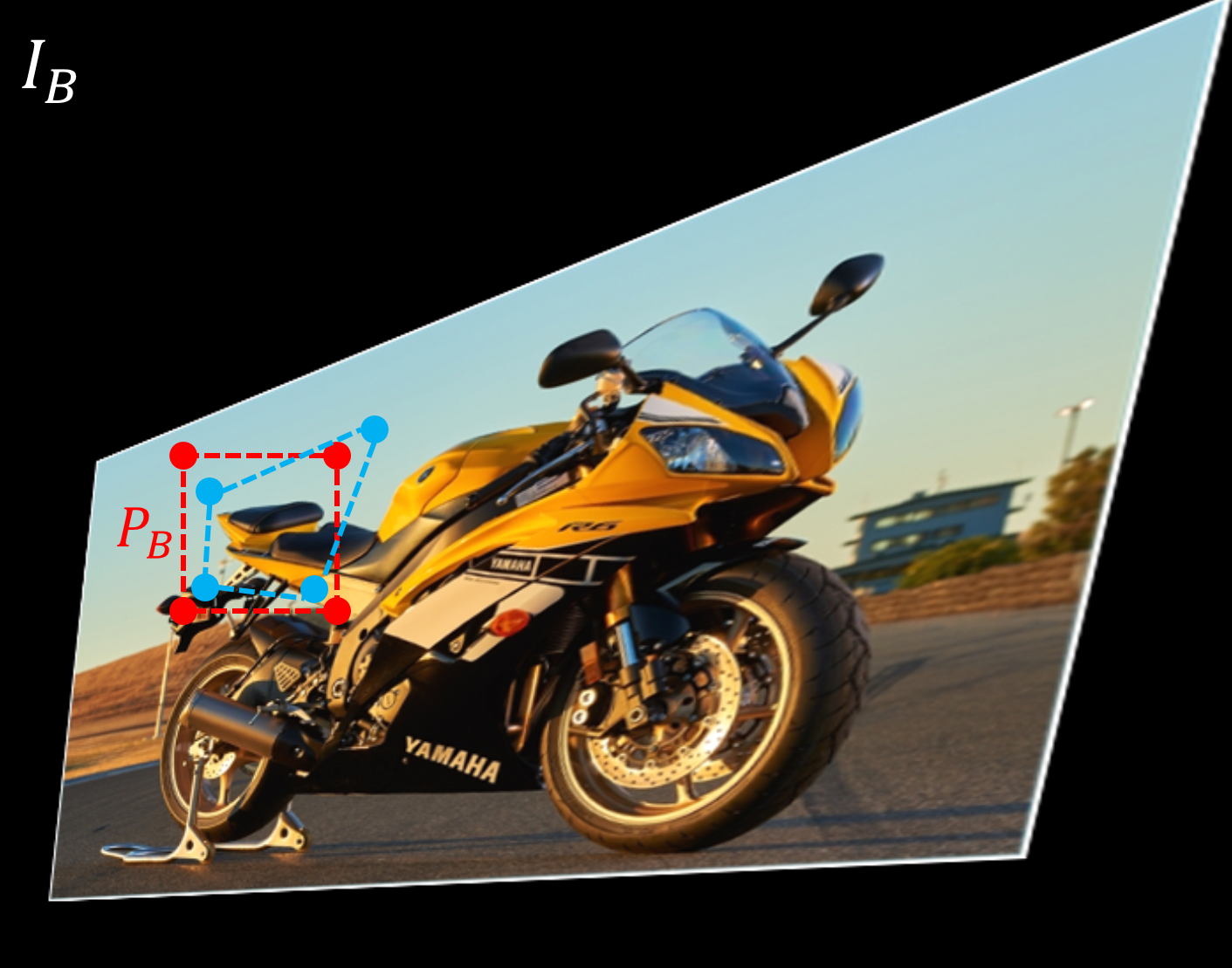
Now, the extracted patches are shown below.
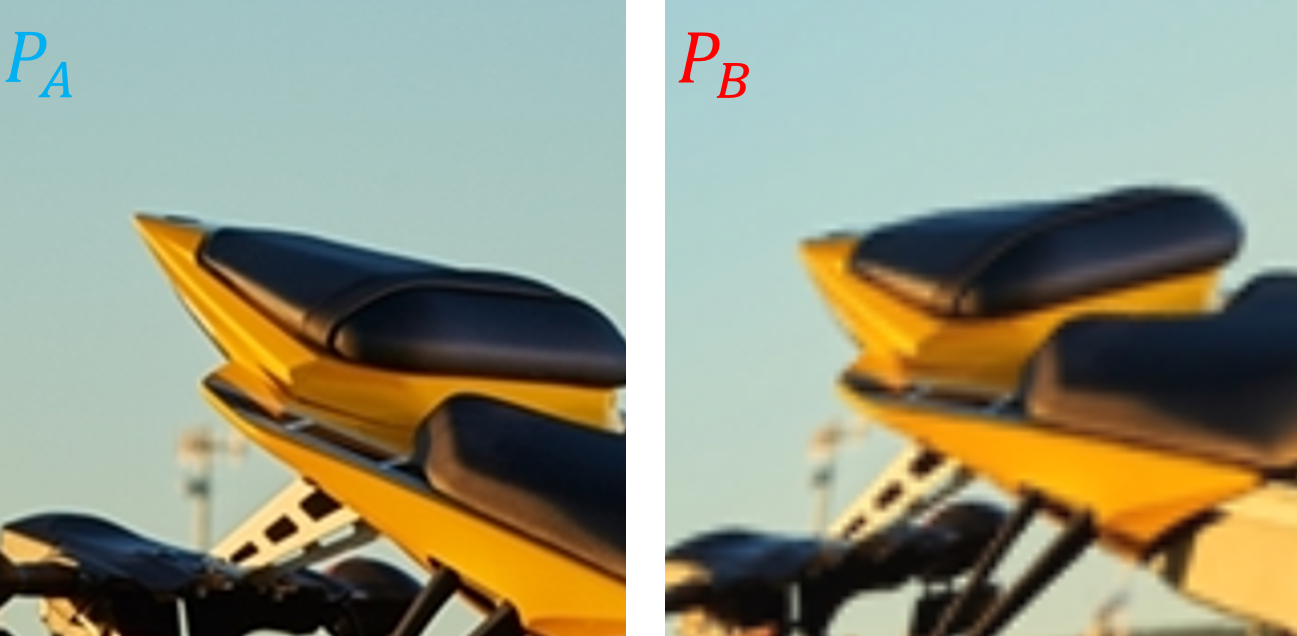
Note that, we generated labels (ground truth homography between the two patches) as is given by \(H_A^B\). However, the authors in this paper found that regressing the 9 values of the homography matrix directly yielded bad results. Instead, another way the authors found was to regress the amount the corners of the patch \(P_A\) denoted by \(C_A\) need to be moved so that they are aligned with \(P_B\). This is denoted by \(H_{4Pt}\) and will be used as our labels. Remember, \(H_{4Pt}\) is given by \(H_{4Pt} = C_B - C_A\).
Now, we stack the image patches \(P_A\) and \(P_B\) depthwise to obtain an input of size \(M_P\times N_P \times 2K\) where \(K\) is the number of channels in each patch/image (3 if RGB image and 1 if grayscale image).
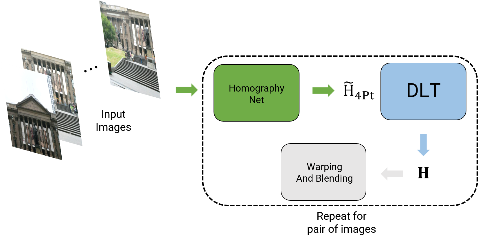
The final output of data generation are these stacked image patches and the homography between them given by \(H_{4Pt}\). An overview of panorama stitching using Deep Learning (both supervised and unsupervised have the same overview) is shown below.
5.2. Supervised Approach
The network architecture and the overview is shown below. However, note that you are free to change the network as you wish.
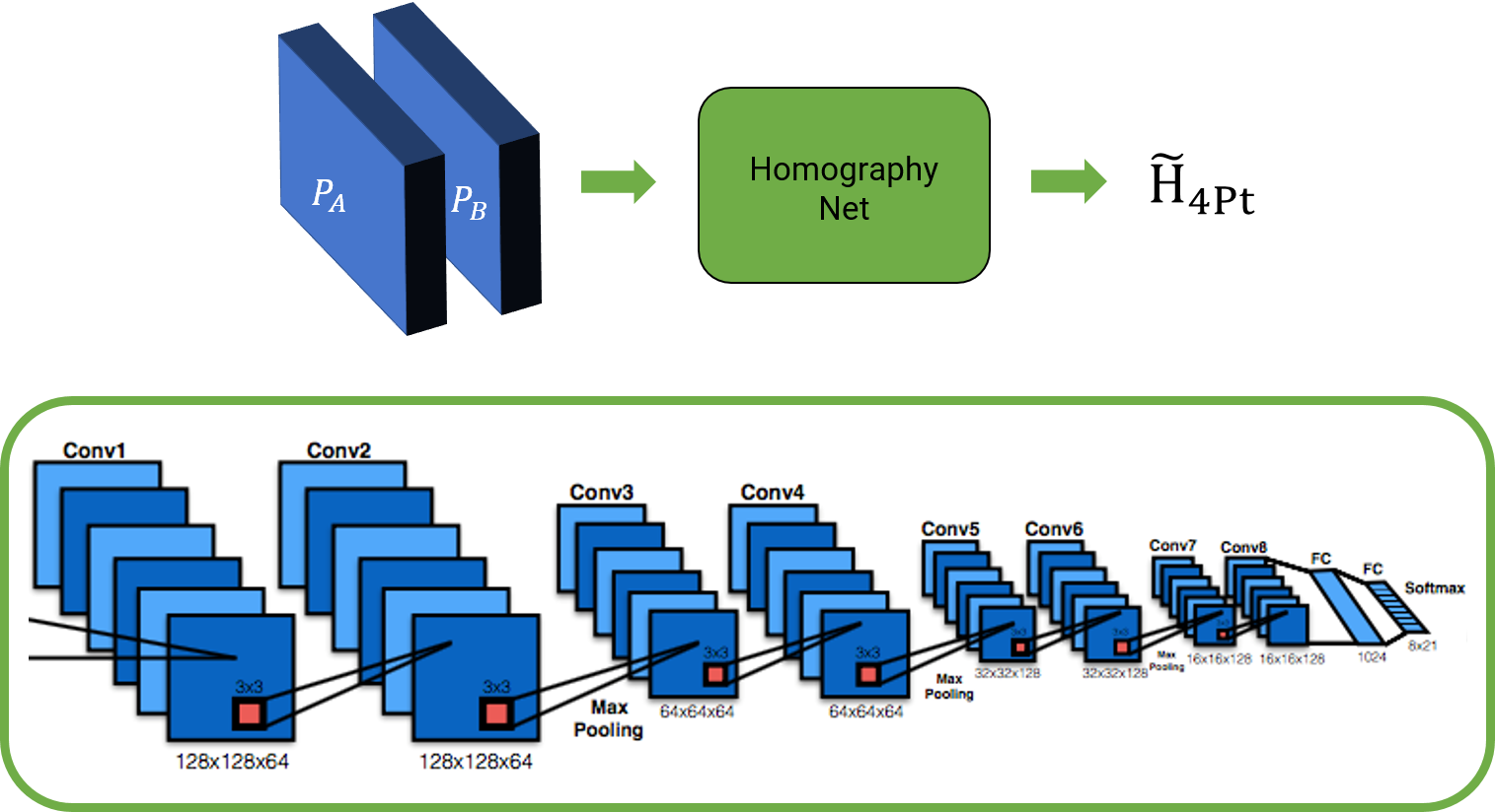
The loss function used is simple L2 loss between the predicted 4-point homography \(\widetilde{H_{4Pt}}\) and ground truth 4-point homography \(H_{4Pt}\). The loss function \(l\) is given by \(l = \vert \vert \widetilde{H_{4Pt}} - H_{4Pt} \vert \vert_2\).
5.3. Unsupervised Approach
Though the supervised deep homography estimation works well, it needs a lot of data to generalize well and is generally not robust if good data augmentation is not provided as shown in this paper. Now, we’ll implement an unsupervised approach to estimate homography between image pairs using a CNN as given in this paper.
The data generation is exactly the same for this part (as we want to evaluate the algorithm later using the labels), note that the labels \(H_{4Pt}\) are not used for learning in the loss function. For the unsupervised method, we want to predict the value of \(H_{4Pt}\) which when used to warp the patch \(P_A\) should look exactly like the patch \(P_B\). This can be written as the photometric loss function \(l\) given by \(l = \vert \vert w(P_A, H_{4Pt}) - P_B\vert \vert_1\). Here \(w(\cdot)\) represents a generic warping function and here specifically warping using the Homography value and bilinear interpolation. Let’s see how we can convert our supervised method into an unsupervised one.
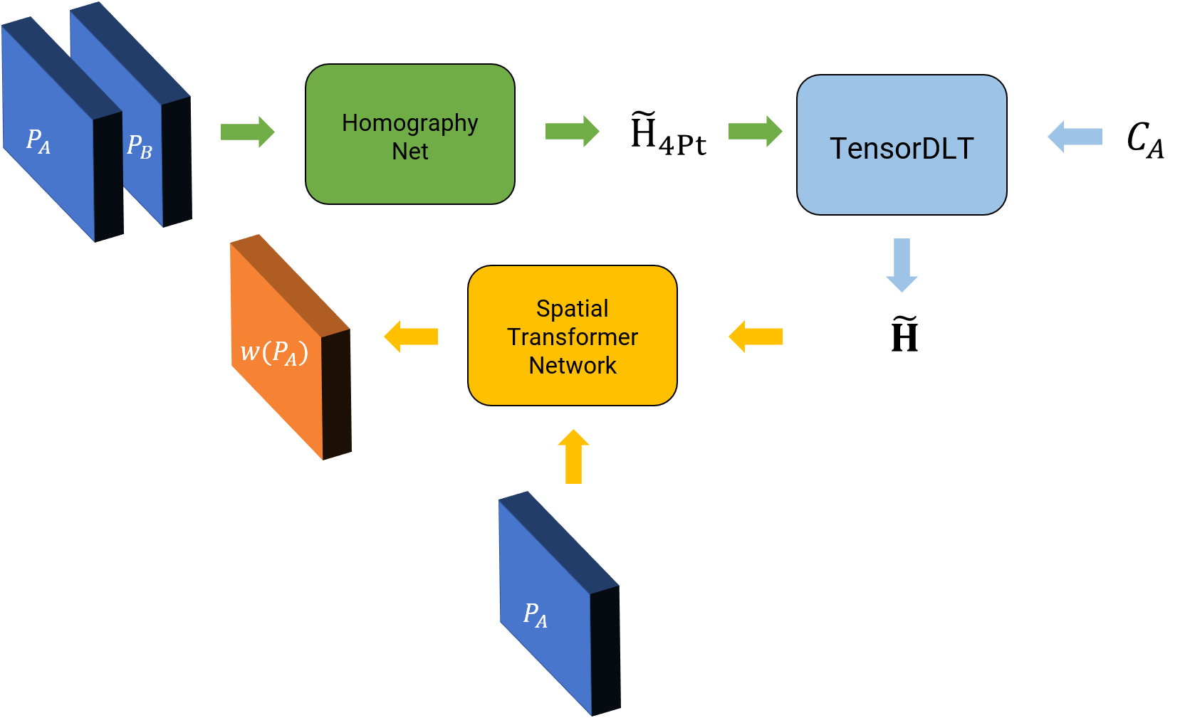
Notice that, now we have two new parts (shown in light blue and yellow in Fig. 17), namely, TensorDLT and the Spatial Transformer Network. The TensorDLT part takes as input the predicted 4-point homography \(\widetilde{H_{4Pt}}\) and corners of patch \(P_A\) to estimate the full \(3\times 3\) estimated homgraphy matrix \(\widetilde{\mathbf{H}}\) which is used to warp the patch \(P_A\) using a differentiable warping layer (using bilinear interpolation) called the Spatial Transformer Network. You need to implement the TensorDLT layer. For further details refer to Section IV B in this paper. A generic Spatial Transformer Network is given to you with the starter code in YourDirectoryID_p1\Phase2\Code\Misc\TFSpatialTransformer.py (you need to modify it as descibed in Section IV C of this paper). Finally, implement the photometric loss function we discussed earlier.
Note that, we didn’t talk about the network architecture here, feel free to use the network you implemented for the supervised version here or be creative.
6. Notes about Test Set
The Test Set can be downloaded from here. The Test Set has the following folder structure.
P1TestSet.zip
|   Phase1
|   ├── TestSet1
|	|	└── *.jpg
|	├── TestSet2
|	|	└── *.jpg
|	├── TestSet3
|	|	└── *.jpg
|	└── TestSet4
|	|	└── *.jpg
|   |
└── Phase2
	└── *.jpg
- Stich Panoramas of images from
Phase1folder using the traditional approach, supervised homography and unsupervised homography. - Use images from
Phase2folder to evaluate your deep learning based homography algorithms (both supervised and unsupervised). Here you can apply random perturbations as before on the center crop of the image (of size you chose during training). This Test is to evaluate how well your algorithm generalized to images outside the training set. (For this part, your algorithm will only run on the image size you chose during training, i.e., \(M_P\times N_P\). A simple way to deal with this is to resize the test image to \(M_P\times N_P\) to obtain the homography and then warp the original image or crop a central region of \(M_P\times N_P\) or obtain random crops of size \(M_P\times N_P\) and average all the predicted homography values. Feel free to be creative here. Mention what you did for this part in your report.)
7. Extra Credit
Implementing the extra credit can give you upto 50% on the bonus score. As we discussed earlier, there is no optimal way to obtain the best homography between two images as we trained our networks on a small patch size. A good way would be to obtain homographies from a lot of patches and then use RANSAC to obtain the best method. We want you to implement this method using deep learning and present a high quality analysis. Refer to the DSAC paper which presents ideas on how to implement RANSAC in a differentiable way for a neural network. You are free to use the DSAC code from the authors to implement this part.
8. Submission Guidelines
If your submission does not comply with the following guidelines, you’ll be given ZERO credit.
8.1. Starter Code
Download the Starter Code for both Phase 1 and Phase 2 from here.
8.2. File tree and naming
Your submission on ELMS/Canvas must be a zip file, following the naming convention YourDirectoryID_p1.zip. If you email ID is abc@umd.edu or abc@terpmail.umd.edu, then your DirectoryID is abc. For our example, the submission file should be named abc_p1.zip. The file must have the following directory structure because we’ll be autograding assignments. The file to run for your project should be called YourDirectoryID_p1/Phase1/Code/Wrapper.py for Phase 1; YourDirectoryID_p1/Phase2/Code/Train.py and YourDirectoryID_p1/Phase2/Code/Test.py for running training and testing models in Phase 2 (the supervised or unsupervised approach will be chosen by the command line flag --ModelType from our autograder). For panorama stitching using deep learning based homography estimation, fill your code in YourDirectoryID_p1/Phase2/Code/Wrapper.py. You can have any helper functions in sub-folders as you wish, be sure to index them using relative paths and if you have command line arguments for your Wrapper codes, make sure to have default values too. Please provide detailed instructions on how to run your code in README.md file.
NOTE: Please DO NOT include data in your submission. Furthermore, the size of your submission file should NOT exceed more than 100MB.
The file tree of your submission SHOULD resemble this:
YourDirectoryID_p1.zip
|   Phase1
|   ├── Code
|   |   ├── Wrapper.py
|   |   └── Any subfolders you want along with files
|   Phase2
|   ├── Code
|   |   ├── Train.py
|   |   ├── Test.py
|   |   ├── Wrapper.py
|   |   └── Any subfolders you want along with files
├── Report.pdf
└── README.md
8.3. Report
For each section of the project, explain briefly what you did, and describe any interesting problems you encountered and/or solutions you implemented. You must include the following details in your writeup:
- Your report MUST be typeset in LaTeX in the IEEE Tran format provided to you in the
Draftfolder and should of a conference quality paper.
Phase 1
- For Phase 1, present input and output images after each section (corner detection, ANMS, feature extraction, feature matching, feature matches after RANSAC) and final panorama for all the Train and Test Images, including the data you collected. The Train images can be found in
YourDirectoryID_p1\Phase1\Data\Train\and the Test set will be released 24 hours before the deadline. Add all the images into yourReport.pdf. - Talk about what you did to blend the common region between images.
- Talk about how you rejected images with no/very less overlap.
NOTE: Test images will be released 24 hours before the deadline.
Phase 2
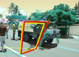
- Present classical feature based (from Phase 1), supervised, unsupervised estimated homographies against a synthetic ground truth for any 4 images from Train/Val/Test set. A sample image is shown below.
- Present the average EPE (average L2 error between predicted and ground truth homographies) results for both supervised and unsupervised approaches along with algorithm run-time for forward pass of the network after the graph has been initialized. Present EPE results on Train, Val and Test sets. EPE is defined as the average of \(\vert \vert \widetilde{H_{4Pt}} - H_{4Pt} \vert \vert_2\) for all the 4 points and all the images.
- Present the network architecture used in your report (a snapshot of the Tensorflow graph will do if the layers are named sensibly).
- Present input and output panoramas using supervised and unsupervised approaches for all the test images from Phase 1’s Test set. You dont need to present outputs of Train set here.
9. Allowed and Disallowed functions
Allowed:
- Any functions regarding reading, writing and displaying/plotting images in
cv2,matplotlib - Basic math utitlies including convolution operations in
numpyandmath tf.layersandtf.nnAPI for implementing network architecturetf.imagefor data augmentation- Any functions for pretty plots
- Any functions for filtering and implementing gaussian blur
- Any function for warping and blending for Phase 1
cv2.getPerspectiveTransformcv2.warpPerspective(For more info, refer: Geometric_Transformations)
Disallowed:
- Any third party code for implementing spatial transformer network (apart from the one given in your starter code)
- Any third party code for implementing TensorDLT (apart from functions specified)
- Any third party code for implementing architecture or augmentation
Kerasor any other layer API
If you have any doubts regarding allowed and disallowed functions, please drop a public post on Piazza.
10. Collaboration Policy
NOTE: You are STRONGLY encouraged to discuss the ideas with your peers. Treat the class as a big group/family and enjoy the learning experience.
However, the code should be your own, and should be the result of you exercising your own understanding of it. If you reference anyone else’s code in writing your project, you must properly cite it in your code (in comments) and your writeup. For the full honor code refer to the CMSC733 Spring 2020 website.
11. Acknowledgements
This fun project was inspired by our research in Perception and Robotics Group at University of Maryland, College Park.